In cyber analytics, the adventure begins by revealing which assets are boldly exposed, which hide in the shadows, and which slip through the network’s labyrinth in disguise.
At 2:13 a.m., the casino’s security team failed to recognize that the fish-tank thermometer, perceived as innocuous, could serve as a point of network access for attackers.
The security team concentrated on camera feeds, payment terminals, and guest records, which were classified as critical assets. In contrast, the thermometer was overlooked and left unprotected.
Accounts of the casino fish-tank breach consistently emphasize the thermometer’s role. The primary lesson is that an ordinary device became the critical access point. The fundamental failure was not a missed patch, but a lapse in attention.
This chapter introduces the basics of network assessment and supplies a roadmap for the discussion that follows. Specifically, before detecting vulnerabilities, mapping attack paths, or evaluating defenses, defenders must address four essential questions:
-
What devices appear to exist on the network?
-
What evidence supports each host’s claim?
-
Which blind spots remain?
-
How much uncertainty attaches to the resulting inventory?
Although these questions appear straightforward, they become complex in Internet of Things (IoT) and Operational Technology (OT) environments. Typically, a complete device inventory is unavailable, and device identities are often ambiguous. Network complexity may obscure devices from detection. Some devices are only recorded in outdated logs, some are easily detectable, others respond selectively to specific probes, and a few remain undetected unless alternative methods are used. Network silence may indicate a missing device, filtered traffic, a limited vantage point, or that certain devices are beyond current detection abilities.
Chapter 1 frames discovery as the process of systematically revealing the network's true composition, acknowledging that certainty is uncommon at the initial stage. This framing establishes the foundation for the chapter’s goals: to highlight that major risks often persist in plain sight while remaining unacknowledged or undervalued. Accordingly, the chapter positions network discovery as the basic step in cyber defense, noting that it is an essential and substantive process rather than a mere preliminary measure. This transition emphasizes the chapter's main objective: constructing a reliable foundation for the following analysis.
This concept establishes the chapter's scope. The objective is to construct a reliable host inventory, differentiate between known and unknown elements, and prepare records for later analysis. To link theory and practice, students are expected to conduct hands-on exercises using the described discovery methods in simulated or real network contexts. Practitioners may adapt these exercises for production networks by limiting discovery runs to specific VLANs or sites, starting with passive techniques before escalating to active probes, and systematically recording both device inventories and visibility gaps. When applying these methods in working environments, coordination with stakeholders, testing during off-peak hours, and documentation of all assumptions regarding network layout and device populations are recommended. Comprehensive identification and vulnerability assessments are addressed in later chapters; at this stage, the attention remains on establishing a firm foundation for further analysis.
Learning Objectives
By the end of this chapter, students should be able to:
-
Explain why network discovery belongs to descriptive analytics rather than scanner operation alone.
-
Describe why IoT and OT environments break the closed-world assumptions common in enterprise vulnerability management.
-
Compare passive, low-disturbance, and active discovery methods in terms of coverage, cost, and operational risk.
-
Explain how topology, privilege, and protocol behavior shape observability.
-
Construct host records as evidence-backed claims with provenance and uncertainty.
-
Evaluate discovery using completeness, soundness, discovery gap, and marginal method contribution.
-
Analyze attacker-defender asymmetry in partially observed environments.
-
State what Chapter 1 hands to Chapter 2, and what remains unresolved at the end of discovery.
1.1 Why Discovery Comes First
A device cannot be secured if it is not included in the inventory.
Caution: The techniques described in this chapter have operational boundaries. Always verify assumptions against the specific deployment environment before relying on any automated output.
In enterprise information technology (IT), that sentence sounds obvious. In IoT and OT, it is a recurrent failure mode. Traditional vulnerability programs often assume a closed world: assets are already known, agent-capable, directory-linked, and recorded in a current management system. Embedded and working environments repeatedly break those assumptions. Devices arrive through facilities teams, contractors, clinical engineering, building management, local purchases, vendor drop-ins, and stale projects that never reached a formal intake path. Some devices speak only on the local link. Others expose narrow protocol surfaces, change names across firmware versions, or cannot host agents at all.
Discovery does not begin with a complete device list. It starts with pieces of evidence and a set of devices yet to be found.
That placement in the analytical sequence matters. A vulnerability inventory can only reason over devices first counted. An attack graph can only model paths through devices first counted. A remediation plan can only govern assets first made visible. When Chapter 1 undercounts the environment, every later chapter inherits the error.
For this reason, discovery is not simply a preliminary step; it constitutes the first substantive action in network management.
This also demonstrates that discovery acts as the foundation for the remainder of the course, establishing the basis for all following analysis.
| Descriptive | What devices exist on the network? | Chapter 1: discovery and inventory |
|---|---|---|
| Diagnostic | What are these devices, and what evidence supports that identity? | Chapter 2: enrichment and fingerprinting |
| Detective | What vulnerabilities or weak configurations do they have? | Chapter 3: Common Vulnerabilities and Exposures (CVE), validation, and credential risk |
| Predictive | Which attack paths are plausible? | Chapter 4: attack-graph reasoning |
| Prescriptive | What actions or tests should be taken next? | Later chapters: offensive testing, remediation, simulation |
Table 1.1. Analytics sequence for the course. Discovery owns the descriptive layer because all subsequent analytical stages depend on the measured host population.
1.2 The Visibility Problem in IoT and OT
The devices most likely to be missed are often the least managed.
This pattern recurs in many incidents, even when the specifics differ. In cases such as Mirai, Verkada, Oldsmar, the Target breach, and the casino thermometer, a device that appeared unimportant or was poorly managed ultimately provided attackers with greater access than anticipated.
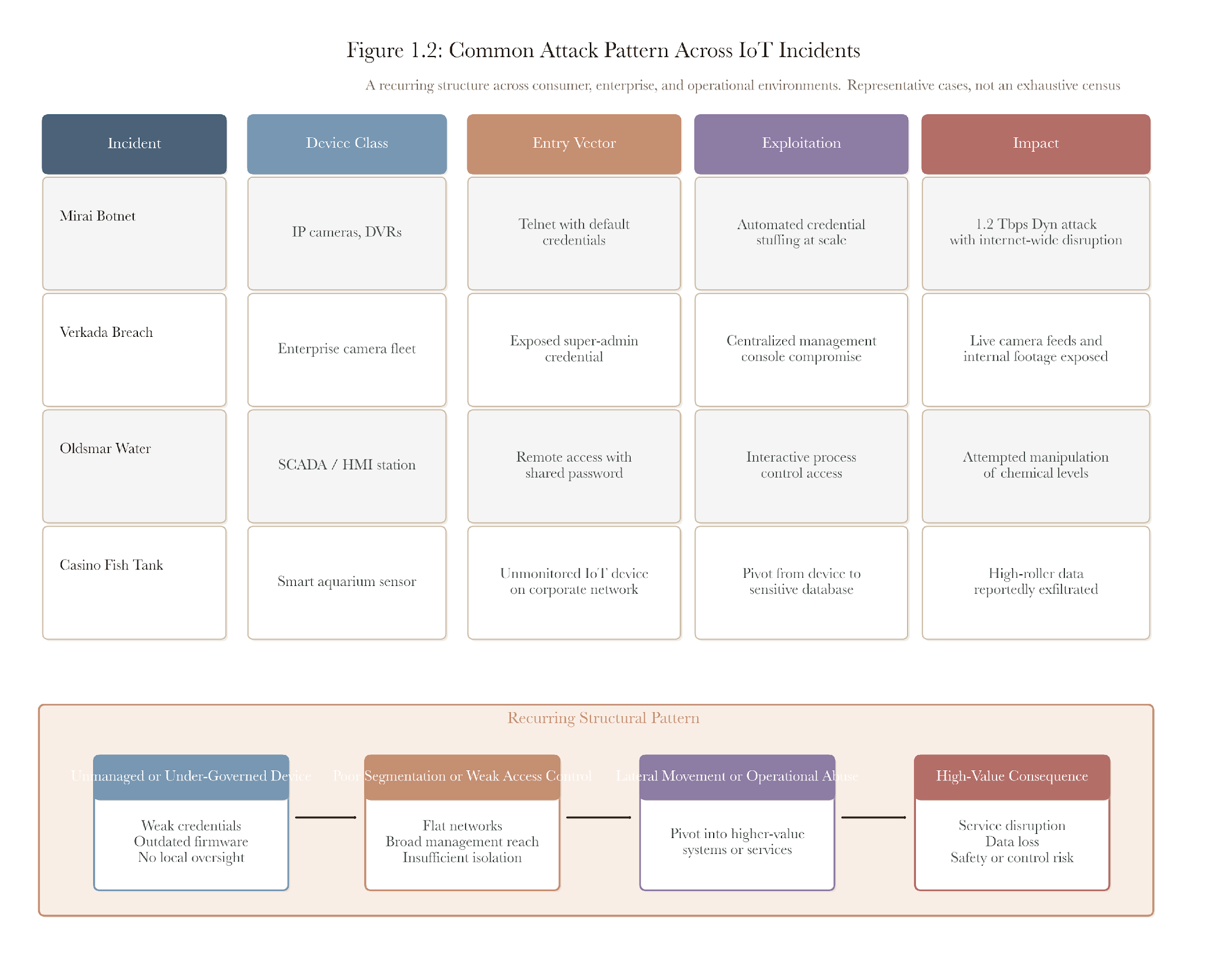
Figure 1.1. A common attack pattern in Mirai, Verkada, Oldsmar, Target, and the casino breach is that a weakly governed edge device or management interface becomes the entry point into more critical systems.
| Mirai | Cameras and digital video recorders |
|---|---|
| Verkada | Managed camera platform |
| Oldsmar | Supervisory control and data acquisition (SCADA) or human-machine interface |
| Target | Heating, ventilation, and air conditioning systems |
| Casino thermometer | Smart environmental device |
Table 1.2. Incident pattern. Different sectors and device classes exhibit the same pattern: weakly governed infrastructure becomes strategically important once it sits on an attack path.
Mirai did not need a subtle foothold. It exploited a vast supply of embedded systems, exposing Telnet and accepting default credentials. Its strength came less from technical novelty than from the scale of unmanaged, reachable devices.
The Verkada compromise demonstrated a different version of the same visibility problem. The devices were known in one sense, but they were not governed as a fleet with a centralized blast radius. Once a privileged credential was abused, cameras installed as local physical-security assets behaved more like a globally reachable surveillance substrate.
Oldsmar and Target matter because they show the same structural weakness outside consumer IoT. In both cases, the dangerous device was not “important” in the way executives usually rank systems. It was important because it sat on a path. A building system, a remote-access workstation, or a heating and ventilation vendor link can become strategically central the moment segmentation and asset awareness fail.
Discovery is the point at which these devices are either managed or remain unnoticed. The goal is to approach enumeration as a visibility challenge, rather than simply a matter of tool selection.
1.2.1 What Discovery Would and Would Not Have Addressed
The control boundary matters. Discovery is necessary in these cases, but it is not sufficient on its own. After devices are discovered and added to the inventory, effective security relies on a series of follow-on controls and processes: asset classification, ownership assignment, vulnerability assessment, persistent monitoring, network segmentation, and ongoing governance to help ensure devices remain visible and managed throughout their lifecycle. Discovery sets the conditions for these additional measures; without visibility, no downstream process can operate effectively, but visibility alone does not guarantee control or safety. Practitioners should recognize that discovery is the basic step, enabling the organization to implement these subsequent protective and governance actions.
| Mirai | Cameras and digital video recorders | Telnet plus default credentials | Population and exposure visibility | Vendor firmware hardening |
|---|---|---|---|---|
| Verkada | Managed cameras | Centralized privileged credential | Fleet scope and blast-radius visibility | Secret management and access control |
| Oldsmar | Supervisory control and data acquisition (SCADA) or human-machine interface | Remote management plus shared credentials | Exposed-interface inventory | Segmentation and multifactor authentication |
| Target | Heating, ventilation, and air conditioning systems | Contractor access and cross-zone pivot | Cross-zone device mapping | Segmentation and least privilege |
| Casino thermometer | Smart environmental device | Flat network and weak defaults | Precondition visibility | Segmentation |
Table 1.3. Counterfactual analysis of what discovery would and would not have invalidated. Keeping the control boundary explicit makes the chapter stronger, not weaker.
Operational importance and analytic visibility frequently diverge. A thermostat, camera, badge reader, operator display, infusion pump, or smart screen may sit at the edge of a procurement workflow while near the center of an attack path. This gap grows with modern device fleets. Devices are often bought outside normal IT processes. Vendors use different names, updates are manual or inconsistent, and protocols vary by vendor and firmware. Ownership records are scattered among departments. What seems like bad documentation locally can become a big measurement problem across the whole network.
1.2.2 Why Traditional Scanners Fail Here
Conventional enterprise scanners remain effective for managed servers and workstations, but they encounter recurrent limits in IoT and OT environments for several compounding reasons:
-
No agent support. Many embedded systems cannot host endpoint agents at all.
-
Protocol diversity. Devices commonly live on multicast Domain Name System (mDNS), Simple Service Discovery Protocol / Universal Plug and Play (SSDP/UPnP), Real Time Streaming Protocol (RTSP), Open Network Video Interface Forum (ONVIF), Message Queuing Telemetry Transport (MQTT), Constrained Application Protocol (CoAP), or related protocol surfaces rather than on the narrow unicast patterns conventional scanners prefer.
-
Identification is inference, not lookup. In unmanaged fleets, identity must often be reconstructed from Organizationally Unique Identifier (OUI) prefixes, hostnames, banners, port signatures, and protocol responses, rather than being read from an authoritative inventory.
-
Topology constrains visibility. Address Resolution Protocol (ARP) does not cross routers. Simple Network Management Protocol (SNMP) needs credentials. Multicast discovery stays local. Each fallback alters not only coverage but also the quality of the evidence.
-
Downstream vulnerability matching depends on the quality of prior discoveries. If the device is never correctly entered into inventory, later Common Platform Enumeration (CPE), CVE, or credential analysis starts from the wrong population.
This does not mean enterprise scanners are useless. It means their usual assumptions do not fit the environments we are discussing here. The environment should guide the sensible choice of tools and methods: in enterprise IT, agent-based or credentialed scans may suffice for managed servers and workstations, while in IoT and OT settings, a mix of passive observation, infrastructure queries, and targeted active probes is necessary. Selection should consider available privileges (such as SNMP or router access), device types present (embedded devices, sensors, cameras, or workstations), and operational sensitivity to scanning. Combining techniques—such as passive ARP, mDNS, SNMP where available, and cautious TCP probing—improves coverage and reduces blind spots. Practitioners should adapt their discovery approach based on what is both observable and permitted, rather than relying on a single tool across all environments.
To keep the chapter concrete, we will follow one device from the first hint of its existence to the Chapter 1 handoff. Students will trace, step by step, how evidence accumulates for this sample device, following the chapter’s structure. This approach clarifies expectations and supports active learning by allowing students to see how each investigative method contributes to building a justified host record.
In our running case, a single entry appears in the local state:
? (192.168.86.42) at d4:f5:47:xx:xx:xx on en0 ifscope [ethernet]. This line indicates that something was recently on the local subnet, but it does not identify the device. At this point, we only have a weak indication that the host exists.
We will come back to this host when we gather more evidence. By the end of the chapter, we will have more information, but we still might not know exactly what the device is. That meticulous approach is important. The goal is to have a reliable record, not to jump to conclusions.
1.4 Discovery as a Measurement Problem
It is a mistake to view discovery as simply running a scanner to obtain a list.
The correct approach is more complex. Defenders gather partial evidence, combine multiple perspectives, estimate what is visible, and consider what may remain hidden. The true device population is D, but the defender does not directly observe D. Instead, the defender sees method-specific subsets:
M1, M2, ..., Mk
Each Mi is determined by topology, privilege, protocol support, timing, device behavior, and network state. The discovered population is the union:
D_hat = union(M1, M2, ..., Mk)
The notation is easy. The inference problem is not. The complement D - D_hat is unobserved by definition. That unseen residue is the discovery gap.
Coverage always depends on the situation. Saying you have “95 percent coverage” only means 95 percent for a specific setup, network layout, timing, methods, and traffic limits.
Silence can mean many things. A device might be missing because it does not exist, is blocked by filters, only responds locally, the scanner used the wrong interface, or due to bad timing.
A host record is an evidence-based claim, not a guaranteed fact. It should include the evidence source, the time observed, and any known issues, as later analysis depends on both what was found and how it was found.
The quiet device at 192.168.86.42 enters the story here as d_hat_1, a candidate member of D_hat supported by one evidence source. That is enough to justify follow-on observation. It is nowhere near enough to justify identity.
1.4.1 What Counts as Discovery Evidence
A reasonable question is whether any network hint is sufficient to create an inventory entry. It is not. Discovery evidence varies in strength depending on how it was obtained and how easily it can become stale, spoofed, or misinterpreted.
The chapter uses the term “host claim” intentionally. A host claim asserts that an addressable device likely exists within the target scope. It does not yet specify the device model, vulnerabilities, or justify remediation. Those determinations require stronger evidence and are addressed in later chapters.
The following evidence classes are useful in Chapter 1:
| Local cached state |
|---|
| Infrastructure state |
| Local-link self-description |
| Active liveness |
| Service evidence |
Table 1.4. Evidence classes for Chapter 1. The classes separate host-existence evidence from later identity and vulnerability evidence.
The table is intentionally cautious to avoid treating all evidence equally. A stale ARP entry, a router observation, a TCP connection, and a service banner each provide information, but their strengths vary.
1.4.2 Negative Evidence Is Not Absence
The second question a reader usually asks is simpler: if a device does not answer, is it absent? In IoT and OT networks, the answer is often no.
Negative evidence is useful only when the method could have seen the device, assuming the device existed and behaved normally under the scan conditions. That condition breaks often. ARP cannot see across a router. mDNS cannot cross a multicast boundary. ICMP can be blocked. TCP probes test only the ports selected. A quiet device behind a gateway may be alive while every local method fails from the scanner’s position.
This is why Chapter 1 avoids expressions like “the subnet is clean” after a quiet scan. A more accurate statement is: “The methods used from this position did not find any hosts during this time.” While less dramatic, it is defensible.
1.5 Observability Depends on Vantage Point
Methods do not simply differ in speed or implementation. They differ in what kinds of worlds they can see.
Local ARP cache harvest sees recent Layer 2 state on the local subnet. Router ARP can extend visibility beyond the local broadcast domain if the defender can query the gateway. mDNS surfaces devices that voluntarily advertise themselves on the local link. Simple Service Discovery Protocol (SSDP) evidence can later corroborate known hosts during enrichment. ICMP and TCP probing can elicit responses from hosts that never self-describe. SNMP can expose network state through managed infrastructure when access is available.
The same network can appear very different depending on whether you use a laptop on Wi-Fi, a scanner on a switch port, a host with gateway access, or a collector over a VPN. Always consider your scanning position when interpreting discovery results.
If you can only see the quiet device via local ARP and not anywhere else, it tells you not only about the device but also about your position in the network and its limits.
The same logic extends to Internet Protocol version 6 (IPv6), even though this chapter stays focused on Internet Protocol version 4 (IPv4). IPv6 discovery replaces ARP with Neighbor Discovery and changes the multicast surfaces involved. However, it does not remove the core problem: visibility is still constrained by vantage point, protocol behavior, and control-plane scope.
The practical version of the vantage-point question is, “Where should the scanner stand?” No universal answer exists, but some choices are better than others for a given claim.
| Analyst's laptop on a wireless subnet | Local ARP, mDNS advertisements, TCP responses from reachable peers | Routed segments, isolated wired devices, gateway-only views |
|---|---|---|
| The host is attached to a switch port in the target segment | Local ARP, low-disturbance local-link evidence, active probe responses | Devices behind other routers or access-control lists |
| Gateway or router with management access | ARP and neighbor tables across served segments, SNMP observations | Application identity, unless service probes are also run |
| Central scanner across a VPN | Routed TCP and ICMP evidence, reverse Domain Name System names were maintained | Local-link evidence, media access control visibility, multicast behavior |
| Distributed collector inside a remote segment | Local-link evidence from the remote segment without moving the central scanner | Requires deployment, registration, and trust in the collector |
Table 1.5. Vantage-point matrix. The same network can produce different evidence depending on the scanner's position.
This matrix is important because it helps analysts avoid overinterpreting clean results. For example, a central scanner may be effective at checking TCP connections across routes but may miss local-link details. A laptop might detect mDNS from a smart speaker but miss devices on another VLAN. A router may know a MAC address but not the device type.
In the Breakwater implementation, this distinction appears as a topology setting rather than a philosophical aside. BREAKWATER_SCAN_TOPOLOGY=auto lets the pipeline decide whether a batch is local or remote. Local forces local-link behavior. Remote skips local-link adapters and relies on routed methods such as TCP probing, ICMP sweeps, reverse name lookup, router state, and agent dispatch, where configured. The setting does not create visibility on its own. It tells the scanner which forms of visibility it can assume.
The rationale for beginning discovery with passive or minimally intrusive methods rests on both analytical sturdiness and operational prudence. Passive-first ordering reduces the risk of inadvertently affecting sensitive devices or critical business operations, especially in environments such as hospitals or manufacturing plants, where even low levels of unsolicited network traffic can pose operational risk. Analytically, starting with evidence that does not generate new traffic—such as harvesting ARP caches or querying existing infrastructure state—provides a baseline of device visibility with minimal confounding factors introduced by the measurement process itself. This sequence allows defenders to establish what is already observable without interference, reducing the risk of misattributing device presence or absence to active scanning. By escalating only when passive methods leave important uncertainty unresolved, practitioners can better attribute the source and meaning of new evidence. This disciplined order also supports clearer interpretation: the appearance of a device in passive data versus only after active probing can inform later analysis about its behavior, presence pattern, and possible operational constraints. Thus, passive-first ordering is not simply a habitual best practice but a principle based on minimizing measurement bias, safeguarding business continuity, and improving the interpretive quality of discovery results.
Discovery should begin with the easiest and least disruptive evidence before generating more intrusive network traffic. This procedure is both practical and analytical. In sensitive environments such as hospitals or factories, unexpected network traffic can cause issues. Even in less critical settings, starting with passive or low-impact evidence provides defenders with better insight before active scanning begins.
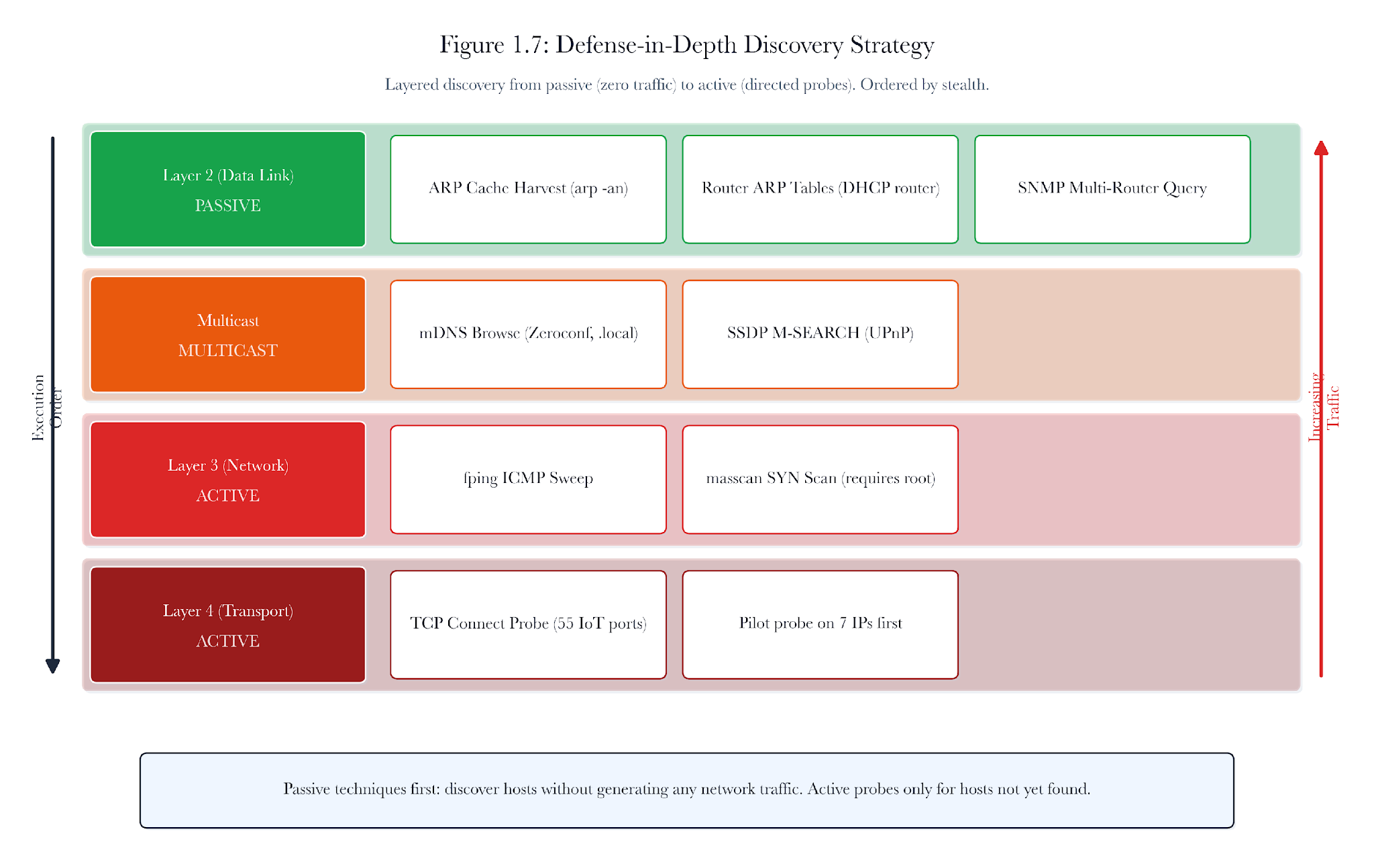
Figure 1.2. Passive-first discovery ordering. Read existing state first, use low-disturbance control-plane and multicast evidence second, and escalate to host-directed active probes only after cheaper evidence has been exhausted.
The ordering used in this chapter is:
-
Read state already present on the local host or gateway.
-
Use a low-disturbance control plane and local link discovery where available.
-
Escalate to active host-directed probing when earlier methods leave important uncertainty unresolved.
This order also clarifies later findings. If a host appears in the ARP cache before any active scans, it was already active on the network. If it only appears after active probing, that indicates a different presence pattern.
Passive-first does not mean using only passive methods. It means starting with the safest options and using more intrusive methods only if questions remain. This is about sound measurement practice, not simply right or wrong.
| Existing local state | Has this host appeared in recent local mappings? | No new target traffic | Recent local evidence exists | Cache may be empty or stale |
|---|---|---|---|---|
| Gateway or managed infrastructure state | Did the infrastructure observe the host? | Management-plane query | Stronger scope if the gateway is authoritative for the segment | Access or scope may be missing |
| Local-link advertisements | Did the device announce itself nearby? | Low-disturbance multicast observation or bounded local exchange | Rich hint about the service family | Multicast may be filtered, routed wrongly, or quiet |
| ICMP or TCP liveness | Does a direct probe elicit a response? | Active host-directed traffic | Stronger existence claim tied to a response | Filtering and port choice limit interpretation |
| Service scan | What reachable service surfaces exist? | More active, Chapter 2 boundary | Evidence for enrichment and identity work | Still no proof of safe absence |
Table 1.6. Passive-first ordering. The interpretation of a positive or negative result depends on the method's traffic posture.
The table also shows why there is no single 'best scanner.' The right method depends on the specific problem. If your inventory is outdated, local and router evidence might be most useful. If a camera blocks ICMP, TCP connect probing on certain ports could help. For devices like Chromecasts or printers, local-link service announcements might provide the key clue.
In our example, starting with passive methods keeps the process organized. The first ARP observation is kept even after active probing starts. It stays in the record and affects how we interpret later evidence. Active evidence does not replace passive evidence; rather, it relies on it.
1.7 ARP Cache Harvesting
Reading the ARP cache is the best initial step on a local IPv4 subnet because it leverages information the operating system already maintains.
1.7.1 Why ARP Matters
On a local segment, ARP provides a mapping between an Internet Protocol address and a media access control (MAC) address. That gives the discovery engine three useful things immediately: recent host activity, by implication; a link-layer identifier; and a path to vendor annotation through the IEEE Organizationally Unique Identifier (OUI) registry.
This initial check does not generate any new packets from the host.
In IoT and OT settings, this first look is often very useful. Devices like cameras, printers, badge readers, smart displays, gateways, thermostats, and appliances near PLCs usually have stable MAC addresses and send small bursts of traffic, even if they reveal little else.
1.7.2 Implementation Choice: arp -an
The implementation uses arp -an instead of arp -a to avoid slow reverse DNS lookups. This may seem minor, but it follows a bigger rule: discovery should not get bogged down in slow name resolution before confirming a device exists.
The adapter in apps/api/app/scanning/arp_adapter.py is intentionally modest. It locates the platform ARP binary, runs a bounded command, parses IPv4 and MAC fields with a regular expression, and returns a dictionary keyed by IP address. If the binary is missing, if the command fails, or if the timeout expires, the adapter returns no observations rather than stopping the scan.
This approach to handling failure is important for learning. ARP is helpful but not essential. If a discovery system fails because one tool is missing, a minor issue becomes significant. It is better to note that ARP provided no data and proceed to the next method.
1.7.3 Normalization and Merge Readiness
MAC addresses should be standardized before OUI lookups or data merging across several methods. Operating systems format MAC addresses differently, sometimes omitting leading zeros or changing separators. Skipping this step can result in mistaking two records for different devices when they are the same.
The adapter adds leading zeros and converts MAC addresses to uppercase before checking the vendor. For example, c:ae:7d:1:2:3 becomes 0C:AE:7D:01:02:03. This is not just for looks. If one method uses the short form and another the padded form, you might think they are different devices. Careful normalization is key to good inventory work.
Vendor information has limitations. An OUI indicates the company that owns the prefix, but does not confirm the product model, firmware, owner, or device type. For example, a Google prefix could appear on a speaker, display, router, or media device. Sometimes, the vendor prefix is missing, locally assigned, randomized, or hidden by virtualization. In Chapter 1, OUI serves only as a vendor hint, not a full device identity.
1.7.4 Limits of ARP
ARP provides evidence only for the local subnet and does not function across routers. It depends on recent network activity and cache retention. An empty ARP cache may indicate a quiet subnet, a recent device reboot, poor timing, or a lack of traffic to update the cache.
Mixed mobile networks add a new identification wrinkle: MAC randomization. Phones and laptops increasingly use locally administered Wi-Fi MAC addresses that do not map cleanly to a stable IEEE OUI. For fixed IoT and OT devices, this rarely matters; on mixed user-device segments, it weakens vendor inference and leaves ARP-only evidence less informative than it first appears.
Some IoT devices are designed to be intermittent. Battery-powered sensors, low-power radios, and infrequently communicating devices may appear in the cache only briefly. In these cases, ARP is helpful but should be viewed as timing-dependent evidence rather than proof of constant presence.
For the running case, ARP yields the first evidence line:
ip: 192.168.86.42
mac: d4:f5:47:xx:xx:xx
source: arp_cache
status: host probably exists on local subnet
This is an improvement, but it is insufficient for device identification. The next step is to determine if the device can be found beyond the local cache.
1.8 Router ARP, DHCP, and SNMP
When local ARP cannot see beyond the broadcast domain, the gateway often becomes the next useful witness.
1.8.1 Router ARP as Cross-Subnet Evidence
A router’s ARP or neighbor table can expose devices on adjacent segments with far less traffic than broad sweeps across every address on every remote subnet. In practice, this can extend visibility from “what my host saw recently” to “what the gateway saw recently.”
If 192.168.86.42 appears in both the local ARP table and the router’s table, the existence claim becomes stronger. If it appears only locally, the claim remains local and potentially transient.
That matters especially on segmented IoT and OT networks. Building-management devices, laboratory instruments, wireless bridges, and vendor-managed appliances may never talk directly to the scanning host while remaining fully visible to the default gateway or Layer 3 switch that serves their segment.
1.8.2 SNMP as an Infrastructure View
Where management access is available, SNMP can expose IP-to-MAC mappings, interface state, forwarding information, and other control-plane observations that a scanner cannot gather from end hosts alone. In this codebase, the router path lives in dhcp_router_adapter.py and snmp_adapter.py, which query ipNetToMediaPhysAddress rather than assuming end hosts will volunteer clean identity data. This does not eliminate uncertainty, though. SNMP-derived visibility still depends on device support, access configuration, and the scope of the queried infrastructure.
In practice, this makes SNMP one of the highest-value discovery methods in managed environments and one of the least available in ad hoc ones. The method is powerful precisely because it shifts the vantage point from endpoint behavior to infrastructure state.
1.8.3 Dynamic Host Configuration Protocol (DHCP) Router Integration
In smaller networks, especially homes, labs, classrooms, and small offices, the defender may not have enterprise SNMP access. The codebase, therefore, includes a router integration path in apps/api/app/scanning/dhcp_router_adapter.py that attempts to recover useful host evidence from the local router without assuming a full enterprise management plane.
The adapter’s auto method tries strategies in the following order: router ARP and reverse name lookup, SNMP when a community string is configured, and Secure Shell access for router platforms that expose lease files. The Secure Shell path looks for common lease file locations such as /tmp/dhcp.leases and /var/lib/misc/dnsmasq.leases. Those paths are implementation details, but they teach a larger point: discovery often has to fit the environment it's in, not the clean architecture diagram.
Gateway choice is also explicit. apps/api/app/scanning/config.py detects the default gateway from the routing table when BREAKWATER_DHCP_ROUTER_IP is not set, then falls back to 192.168.86.1. That fallback is useful for a common residential-style lab, but it is not evidence. If the gateway's guess is wrong, the router adapter may contribute nothing or data based on the wrong administrative assumption. A serious field run should record the gateway, method, credentials used, and subnet scope.
1.8.4 Topology-Sensitive Method Choice
Method choice ought to follow network status rather than habit. A workstation without gateway visibility should not behave as though it can see a routed enterprise the same way an instrumented gateway can. Discovery results carry the shape of the vantage point that produced them.
If router ARP confirms the same MAC on the same subnet, the claim now has two independent observations tied to the recent network state. The first ARP entry was not a single artifact.
If the router's ARP table conflicts with the local ARP table, the discrepancy calls for attention. It may mean a stale local cache, a reused address, a virtual interface, a moved device, or a network address translation artifact. A polished report should not hide the conflict by silently choosing one value. It should retain both observations, including their timestamps and source labels, until the conflict is resolved.
In operational practice, this means that when conflicting evidence is detected, analysts should first flag the discrepancy in the host record and document both the sources and the time of observations. The next step is to triage the conflict by reviewing recent network events, device movement, and DHCP or routing changes to determine the likely cause. Stakeholders may need to validate the device’s current state via manual inspection or coordinated queries. Finally, the resolution process and outcome should be clearly logged, so that subsequent audits or computerized systems can learn from past reconciliation efforts. This deliberate approach facilitates maintaining a defensible, auditable inventory, making sure that unresolved conflicts are visible and actionable rather than dismissed in silence.
1.9 Local-Link Discovery and Self-Description
Some of the most useful IoT evidence is announced to nearby peers rather than exposed to generic remote scanners. The implementation boundary matters here. In Breakwater, mDNS browsing can discover hosts by listening for local-link advertisements without starting from a known IP list. SSDP is enabled in configuration, but the adapter in apps/api/app/scanning/ssdp_adapter.py probes known IP addresses during enrichment. Chapter 1, therefore, treats SSDP as local-link evidence that can corroborate and explain an admitted host claim, not as the primary host-admission mechanism in the progressive discovery phase.
1.9.1 mDNS
mDNS can reveal hostnames, service types, and local-link identity for devices that participate in zero-configuration ecosystems. It is especially valuable because it often surfaces semantically rich hints that raw ARP cannot provide.
In practice, multicast traffic on User Datagram Protocol (UDP) port 5353 may reveal far more to the defender than an ICMP echo ever will. A response advertising _googlecast._tcp, _airplay._tcp, _ipp._tcp, or _printer._tcp is not yet a full device identity, but it is already a richer observation than “host responded.”
In real fleets, those service strings change the next question. Chapter 1 records that the host advertised a service type and therefore deserves enrichment. Chapter 2 decides what identity claim, if any, follows from that service string.
The repository’s mDNS adapter makes this distinction visible. apps/api/app/scanning/mdns_adapter.py maintains a list of service types common in consumer and small-office devices, including Google Cast, AirPlay, HomeKit, Internet Printing Protocol, printer, Real Time Streaming Protocol, Sonos, Spotify Connect, Server Message Block, and Secure Shell advertisements. During browsing, it starts Zeroconf service browsers, waits for the configured browse window, resolves advertised service records, and keeps fields such as device_name, model, manufacturer, device_type_hint, hostname, and advertised services.
Those fields should still be handled carefully. A device name may be user-assigned. A model field may be absent. A service type can describe a capability rather than a complete device class. A device advertising _ipp._tcp is most likely a printer, or at least a print-capable device, but Chapter 1 should not convert that service string into an exact model. The disciplined move is to admit the host and preserve the service evidence for Chapter 2.
1.9.2 SSDP
SSDP plays a related role for Universal Plug and Play (UPnP) devices. It can expose device class and service descriptions, sometimes disclosing more about the device family than any low-rate liveness probe could determine.
Here, the relevant control-plane surface is usually User Datagram Protocol (UDP) port 1900 with an M-SEARCH request and a response containing a LOCATION pointer into a UPnP device description. The adapter in apps/api/app/scanning/ssdp_adapter.py sends a bounded unicast M-SEARCH to known IPs, extracts the LOCATION header, and parses the device description with defusedxml.ElementTree. Even at the Chapter 1 scope, that matters because it distinguishes “device exists” from “device exists and is already leaking structured self-description.”
This is especially common in smart TVs, media servers, consumer gateways, network storage, and some camera or network video recorder ecosystems. Even without resolving full identity, a UPnP response can turn a weak existence claim into a more understandable one.
The security detail is also worth noting. UPnP device descriptions are Extensible Markup Language (XML) documents fetched from devices that may be poorly maintained or hostile. The adapter uses defusedxml.ElementTree so that XML parsing does not become an unnecessary parser-risk lesson inside a discovery pipeline. Chapter 1 does not need to score that device yet. It does need to record that the device volunteered a structured description and that the parser treated the response as untrusted input.
1.9.3 Quiet Failure Modes
Multicast discovery has its own traps—interface binding matters. VPN tunneling can redirect packets to the wrong place. A scanner can look healthy while sending discovery traffic through an interface that never reaches the target segment. In this repository, that problem is handled explicitly in mdns_adapter.py via _detect_lan_ip(), which avoids blindly binding Zeroconf to 0.0.0.0 when a tunnel interface hijacks the default route. In discovery, failure is often quiet.
Suppose 192.168.86.42 produces no mDNS response and no useful SSDP evidence during the later known-host probe. That does not prove the device is silent in every sense. It may mean the device does not self-advertise, that our interface is wrong, that the probe path is blocked, or that the relevant exchange did not occur during the observation interval.
Managed switches cause another quiet failure mode: Internet Group Management Protocol (IGMP) behavior can suppress multicast visibility without appearing to be an outright scan failure. That is one reason multicast evidence should be treated as high-value when present and ambiguous when absent.
The record should therefore grow like this:
ip: 192.168.86.42
mac: d4:f5:47:xx:xx:xx
sources: [arp_cache, router_arp]
multicast: no useful response observed
Note: absence of mDNS/SSDP evidence does not resolve device class
The existence claim is stronger, but the device still reveals little about what it is.
1.10 Active Sweeps: fping and masscan
Passive and low-disturbance methods do not finish the job. At some point, the defender has to ask the network direct questions.
1.10.1 fping ICMP Sweep
fping offers cheap, broad liveness testing across a subnet. It is fast and easy to interpret when responses appear. Its weakness is equally plain. Some devices drop ICMP. Some firewalls filter it. Some embedded systems never respond to echo requests, even when they are alive and reachable via other protocols.
If 192.168.86.42 responds to ICMP, the existence claim gains another line of support. If it does not, the right inference is limited: non-response narrows neither existence nor identity by much.
This is a recurring IoT pattern. Many devices are deliberately quiet on ICMP while remaining reachable on Hypertext Transfer Protocol (HTTP), Real Time Streaming Protocol (RTSP), Message Queuing Telemetry Transport (MQTT), or vendor-specific management ports. ICMP is useful as a cheap sweep, not as a decisive absence test.
The implementation keeps the fping role narrow. In apps/api/app/scanning/nmap_adapter.py, the sweep command is:
fping -a -g <subnet> -q -r 0 -t 50
That command asks for alive hosts across a generated address range, uses no retries, and applies a short timeout. The teaching point is not that these exact values are universal. The point is that Chapter 1 should record the traffic policy that produced the result. A host that fails a no-retry, short-timeout ICMP sweep has not failed every possible reachability test. It failed this one.
1.10.2 masscan as Coarse Search-Space Reduction
Masscan is useful for large address spaces because it can identify which subnets deserve more expensive follow-on work. Treated properly, it is a coarse search tool. Treated improperly, it becomes a false oracle.
For Chapter 1, Masscan belongs in the toolbox to reduce search costs, not as the sole source of truth for inventory formation.
That caution is sharper in OT settings than in ordinary enterprise IT. Stateless high-speed probing is attractive on paper and easy to misuse on fragile systems. In sensitive environments, the operational question is never just “will this find hosts?” but also “what traffic pattern can the environment tolerate?”
Breakwater uses Masscan conservatively in discovery. The liveness path probes a small, fixed set of ports (22, 80, 443, 554, 8080) and deduplicates results by IP address. For larger networks, the progressive pipeline can run a single pre-sweep, group responding hosts by /24, and skip full discovery for batches that the pre-sweep found empty, while still retaining local ARP evidence. That design makes Masscan a search-space reducer rather than the final inventory judge.
A subtle reader question follows: if Masscan says no host answered, why not stop? Because stateless scanning loses information under packet loss, filtering, asymmetric routing, and devices that do not listen on the chosen ports. A negative masscan result is a cost signal, not proof that the address space is empty.
1.10.3 What Changes in the Running Case
Suppose ICMP to 192.168.86.42 is filtered, and masscan shows a response only on a small set of common ports. The device is no longer a mere ARP artifact. It has become a host with a specific pattern of reticence: visible enough to confirm, quiet enough to resist easy classification.
The next question is: which service ports will accept a full TCP connection attempt?
1.11 TCP Connect Probing and the Pilot Probe
Some devices reveal themselves only when a connection reaches one of a small number of service ports. TCP connect probing is therefore the durable fallback when passive and low-disturbance methods leave unresolved uncertainty.
1.11.1 Why TCP Connect Matters
A successful TCP connect yields stronger evidence than generic liveness alone because it ties the host to a reachable service endpoint. Even then, an open port is still not a device identity. It is evidence for later chapters.
In IoT and OT practice, the most informative ports are often not the classic enterprise defaults. Web interfaces on 80 or 443 remain common, but so do camera-facing ports such as 554, message-bus ports such as 1883 or 8883, and device-specific management ports that reveal only that something operational is present and listening.
The Breakwater TCP probe list in apps/api/app/scanning/progressive_helpers.py makes that practice concrete. The local list includes core administration and web ports, RTSP on 554, printer ports 631 and 9100, Apple-related ports 3689, 5353, 7000, and 62078, smart television ports 3000, 3001, 8001, and 8002, Sonos ports 1400 and 1443, Google Home and Nest ports 8008, 8443, 10001, 10002, and 10010, network-attached storage ports 5000, 5001, and 445, automation ports 1883, 5683, and 8883, and vendor-specific camera or bridge ports such as 37777, 9998, 9999, and 8081.
The list is not a claim that every such port is safe or complete. It is a defensible compromise: broad enough to catch common embedded service surfaces, narrow enough to remain a liveness probe rather than a full port scan. Chapter 2 can then perform service detection and protocol interpretation on the admitted hosts.
1.11.2 Pilot Probe Strategy
Full-port exploration across large routed address spaces can quickly become expensive. A pilot probe reduces that cost by sampling a small set of addresses and ports first. If a subnet looks empty under a low-cost initial probe, the system can delay more expensive follow-on work. If the pilot finds evidence, the subnet moves up in priority.
The fixed-pilot is a pragmatic heuristic in place of a formal result. Its value is simple: spend more effort where the probability of useful evidence is higher while preserving the option to revisit quiet segments later. In the repository implementation, the heuristic is concrete rather than rhetorical: seven sampled IPs, three ports per sample, and escalation only when those low-cost touches suggest a live subnet.
The pilot also has a visible weakness. A sparse subnet with a single camera at .37, a programmable logic controller at .88, or a building controller at .203 can evade the pilot if none of the sampled addresses or ports answer. The implementation treats the pilot as a cost-control heuristic rather than a proof of space. In a safety-critical or high-priority environment, a quiet pilot should trigger a documented decision: accept the missed-host risk, run a fuller low-rate pass, deploy a local collector, or use infrastructure evidence from routers and switches.
1.11.3 Implementation Grounding in the Breakwater Pipeline
In the repository implementation, this logic is embodied in a concrete progressive pipeline. The orchestration layer builds a ProgressiveScanPipeline, moves method outputs using shared merge state, and emits host records incrementally rather than waiting for a monolithic batch result.
Several implementation choices matter analytically:
-
Local ARP is harvested once near the start of discovery in apps/api/app/scanning/progressive.py and parsed by apps/api/app/scanning/arp_adapter.py through arp -an. The parser zero-pads MAC octets before vendor lookup so that operating-system formatting differences do not create artificial host differences.
-
Router-assisted visibility is handled by apps/api/app/scanning/dhcp_router_adapter.py, which tries configured router strategies and falls back to ARP tables and reverse Domain Name System evidence. This is not the same as claiming that the scanner can see every routed segment from a workstation.
-
SNMP-based remote visibility lives in apps/api/app/scanning/snmp_adapter.py. It walks ipNetToMediaPhysAddress on configured routers and can filter results to the target subnet. It contributes IP-to-MAC evidence when routers and community strings are configured; it is turned off by default.
-
Large-network pruning uses masscan when BREAKWATER_PROGRESSIVE_MASSCAN_ENABLED is true, then falls back to fping when the masscan path is unavailable or fails. The TCP-connect fallback is implemented in apps/api/app/scanning/progressive_helpers.py.
-
The remote TCP pilot is fixed, not adaptive: .1, .10, .50, .100, .150, .200, and .254 are checked on ports 22, 80, and 443 before the full remote port list is attempted.
-
Concurrency is bounded by batch concurrency, enrichment concurrency, and a TCP-probe semaphore. The point is to make earlier evidence available without treating maximum traffic as maximum quality.
The repository also makes these choices explicit in configuration. In .env.example, defaults such as BREAKWATER_ARP_ENABLED=true, BREAKWATER_MDNS_ENABLED=true, BREAKWATER_MDNS_BROWSE_ENABLED=true, BREAKWATER_SSDP_ENABLED=true, and BREAKWATER_DHCP_ROUTER_ENABLED=true encode a local-subnet posture that favors existing state and low-disturbance local-link evidence. The SSDP flag applies to the later known-host adapter, not to primary discovery admission. BREAKWATER_SNMP_ENABLED=false indicates that routed infrastructure visibility is powerful but environment-dependent, while BREAKWATER_PROGRESSIVE_TCP_PROBE_REMOTE=true enables TCP-connect probing when local-link methods cannot be used.
When deploying these settings in production environments, especially within sensitive IoT or OT networks, practitioners should take care to avoid operational risk. It is prudent to review and tune discovery parameters in coordination with operational stakeholders, since aggressive scans or misconfigured active methods can damage fragile or safety-critical systems. Begin with passive and low-disturbance settings, validate operation in a controlled window or test subnet, and escalate to active probing only with stakeholder approval and after reviewing the potential network impact. Always maintain a backup of current configurations, document changes made to scanning profiles, and record the rationale for enabling or restricting specific methods. Production deployments benefit from gradual rollout, targeted scoping (such as per-VLAN or site), careful scheduling, and persistent monitoring for any unanticipated effects. These best practices help help ensure safe and effective discovery by decreasing the risk of unintended disruption.
The implementation files make the same architecture visible in code rather than prose. In apps/api/app/scanning/progressive.py, the pipeline builds shared asyncio queues, harvests ARP once for local topology, runs a large-network masscan pre-sweep when enabled, and gates mDNS browse to local subnets. In apps/api/app/scanning/dhcp_router_adapter.py, the router adapter tries SNMP, then Secure Shell, and finally an ARP-table fallback when the method is set to auto. In apps/api/app/scanning/nmap_adapter.py, the fast-path commands are concrete: masscan probes 22,80,443,554,8080 for reachability, and fping runs as fping -a -g <subnet> -q -r 0 -t 50 when the masscan path does not contribute.
1.11.4 An Illustrative Bound on Discovery Recall
We can sharpen the measurement framing in this chapter without claiming that the resulting model is exact. The point is practical: complementary discovery methods should be justified by marginal gains in visibility, not accumulated by habit.
Consider a network containing N devices and a discovery pipeline using M methods. Let method m detect any given device with probability p_m, where 0 < p_m < 1. Under conditional independence across methods for a fixed device, the expected recall R satisfies:
R = 1 - product over m=1..M of (1 - p_m)
This is not a claim that the methods are truly independent in operational networks. They often are not. It is a baseline showing why partially overlapping methods help so much: each additional method lowers the miss probability multiplicatively rather than additively.
When methods are positively correlated, the independence expression becomes optimistic. In practice, that means the bound should be read as an upper-bound planning approximation rather than as a literal guarantee. ARP and router ARP, for example, are not independent views of the world. They are differently scoped observations of the same network state.
To summarize, the key operational implication for Chapter 1 is that assembling a complementary set of discovery methods—such as ARP, mDNS, router state, SNMP, fping, masscan, and bounded TCP probing—yields broader and more reliable coverage of the device population than reliance on any single approach. While each method may be incomplete on its own, their combined application addresses the blind spots inherent to any standalone technique. Moreover, prioritizing rapid, low-impact evidence sources, such as ARP harvesting, before escalating to more intrusive active probing maximizes coverage efficiency and reduces operational risk. This sequencing helps ensure the discovery process remains both defensible and analytically robust, establishing a firm foundation for all subsequent assessment stages.
This expression is illustrative. The current repository implements a fixed remote pilot, not an adaptive bandit controller. A bandit-style upper-confidence-bound allocator would be a research extension, not a behavior students should assume when reading scan output from the current codebase.
1.11.5 The Running Case Tightens
Suppose TCP connect succeeds on ports 80 and 443 for 192.168.86.42 and fails elsewhere in the first pass. Now the record looks like this:
ip: 192.168.86.42
mac: d4:f5:47:xx:xx:xx
open_ports: [80, 443]
sources: [arp_cache, router_arp, tcp_connect]
icmp: no response observed
multicast: no useful response observed
status: host existence well supported; identity unresolved
The record is much stronger than the one we started with, but it is still incomplete. Converting it directly into a device label crosses the boundary too early.
1.12 Streaming Discovery and Time-to-First-Truth
Discovery should not force the analyst to wait for a monolithic batch result if useful evidence is already present.
1.12.1 Producer-Consumer Structure
As soon as hosts appear, the pipeline can normalize MAC formats, filter obvious artifacts, merge observations, and persist provisional host records. This reduces wall-clock time and improves operator awareness because the inventory begins to form while discovery is still in progress.
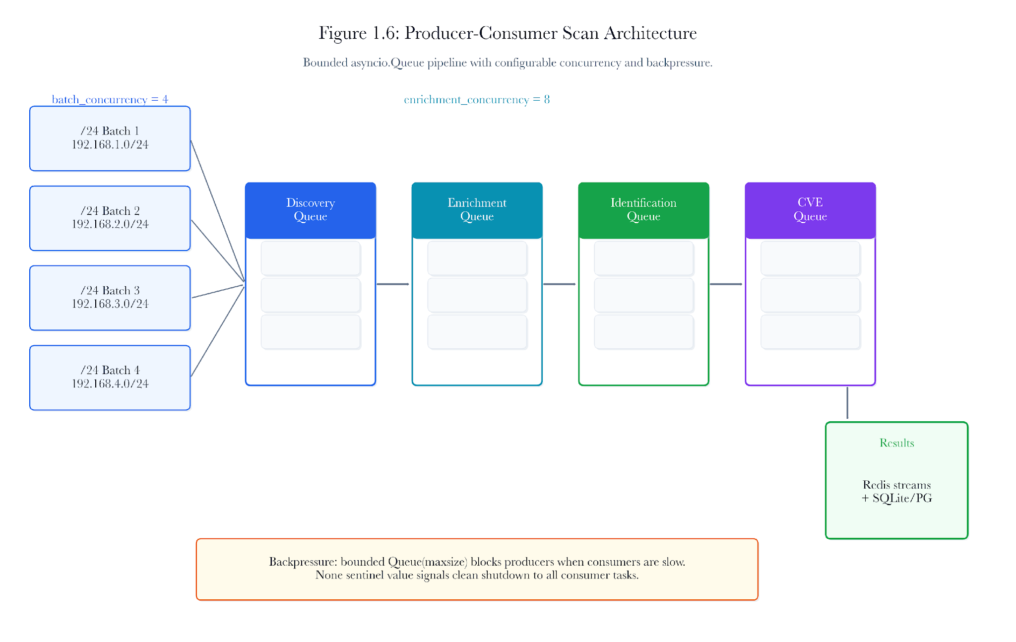
Figure 1.3. Producer-consumer scan architecture. Discovery methods, normalization, filtering, and persistence overlap so that host records appear early while the scan is still running.
In apps/api/app/scanning/progressive.py, this structure rests on three asyncio queues: discovery, enrichment, and identification. Discovery pushes a batch downstream as soon as that batch has usable hosts. Enrichment does not wait for the entire network to finish. Identification does not wait for every enrichment adapter to complete against every host.
That engineering choice has an analytic consequence. The operator sees a moving inventory, not a frozen final truth. Early rows should be read as provisional. A host first admitted by ARP may later gain a hostname from reverse lookup, a service set from nmap service detection, a local-link name from mDNS, or a stronger identity signal in Chapter 2. The row is not wrong because it changes. It is doing what a measurement pipeline should: preserving evidence as it improves.
1.12.2 Bounded Concurrency
Concurrency is useful only up to the point where sockets, CPU, file descriptors, and network disturbance remain under control. The goal is not maximal parallelism. The goal is to obtain evidence earlier and more cleanly.
A global semaphore and bounded worker counts are not incidental engineering choices. They are part of the discovery method itself because they shape traffic rate, timeout behavior, and the reliability of negative evidence.
The default configuration gives that boundary a concrete form: progressive_batch_concurrency defaults to 4, progressive_enrichment_concurrency defaults to 8, and the TCP probe helper uses a global semaphore to prevent the event loop from creating an uncontrolled number of simultaneous connections. The exact values may change by deployment, but the principle should not. A scan that overwhelms the network, the scanner, or the target devices produces bad evidence even when it produces many rows.
The pipeline also stores scan state with a time-to-live key policy when Redis is available. That is not a textbook footnote. Long-running discovery needs a progress state because operators cancel, resume, and inspect scans while they are still in motion. If the student sees a host appear early in the interface, the correct interpretation is “this host has crossed the current admission threshold,” not “all evidence about this host is complete.”
1.12.3 Why Early Partial Truth Matters
A streaming pipeline delivers early partial truth with explicit incompleteness. That is preferable to long silence followed by output that looks final because it arrived at the end.
1.13 Deduplication, Filtering, and Host-Record Construction
Discovery methods do not cleanly partition the device population. They produce overlapping, noisy slices.
1.13.1 Deduplication
The same host may appear through ARP, router ARP, SNMP, mDNS, ICMP, TCP connect, and later SSDP corroboration. The pipeline has to merge those observations into a single host record without erasing provenance.
The merge key in the discovery phase is usually the IP address, since the pipeline is building an addressable host inventory. That choice is practical, but it is not perfect. IP addresses can be reused. Dynamic leases can move. Network Address Translation (NAT) can hide multiple devices behind a single IP address. A MAC address can be unavailable on remote subnets. The analyst should therefore treat IP-based merge as an operational key, not as an ontological proof that the same physical device persisted unchanged over time.
Where possible, host records should retain fields that enable later corrections: IP address, MAC address, hostname, vendor hint, source method, timestamp, open ports, and whether the observation came from local state, infrastructure state, self-description, or active probing. If later evidence contradicts an earlier row, the provenance makes the conflict diagnosable.
1.13.2 Broadcast and Multicast Filtering
Some observations are not hosts at all. They are broadcast addresses, multicast artifacts, relay behaviors, stale cache remnants, or malformed entries. Promotion into the inventory should therefore require more than mechanical collection.
The implementation applies several plain filters before returning a discovery batch. It drops .255 and .0 address artifacts and filters the broadcast MAC address FF:FF:FF:FF:FF:FF. Later, after enrichment, _is_phantom_host() removes entries with no useful identifying signal: no open ports, no MAC address, no hostname, no vendor hint, and no enrichment evidence. These rules are not a full truth model, but they express a sound principle: the inventory should not promote rows that carry no defensible host signal.
1.13.3 Phantom Hosts
Phantom hosts are discovery-specific false positives. They arise when stale state or network artifacts are mistaken for real devices. A noisy Chapter 1 poisons every later chapter because identity, vulnerability, and attack-path reasoning all inherit the same contaminated population.
The false-positive problem isn't only aesthetic. If a phantom host enters Chapter 2, enrichment may waste time probing a non-device. If it enters Chapter 3, a vulnerability report may appear to cover or condemn a host that was never real. If it enters attack-path analysis, the graph may create a path through a node that should not exist. This is why soundness belongs in Chapter 1 rather than in a later cleanup pass.
The opposite mistake is also serious. A strict filter can remove a real but quiet device. Selecting an appropriate filtering policy requires critical reflection regarding the intended use of the discovery inventory. For example, in a research benchmark, it is often advisable to apply strict admission criteria and document the rules explicitly, as this approach clarifies the trade-off between exactness and recall. In operational safety reviews, practitioners should consider introducing an intermediate 'needs verification' category for hosts that possess weak yet plausible evidence, thereby avoiding the unintended exclusion of legitimate yet low-visibility devices. Students should be encouraged to articulate the rationale for their chosen admission policy, customizing it to their analytic goals and operational risk tolerance, and to document both the criteria used and any resulting uncertainties to facilitate transparent and reproducible analysis.
1.13.4 Host Record as an Analytic Contract
The output of Chapter 1 is not whatever the scanner happened to print. It is a structured record that states what can be justified and what remains unresolved.
An illustrative Chapter 1 handoff for the running case might look like this:
ip**:** 192.168.86.42
mac**:** d4:f5:47:xx:xx:xx
vendor_hint**:** Google Inc.
hostname**:** unknown
open_ports**:**
- 80
- 443
discovery_sources**:**
- arp_cache
- router_arp
- tcp_connect
timestamps**:**
first_seen**:** illustrative
last_seen**:** illustrative
confidence_note**:** device existence is well supported; device identity remains unresolved
The record is strong on existence and intentionally weak on identity. That is the correct outcome at this stage.
A reader may still wonder why the record does not simply say “camera,” “speaker,” or “router” once ports and vendor hints appear. The answer is that the Chapter 1 contract is narrower. A camera-like port set can be part of a camera, a network video recorder, a media bridge, a test container, or a vendor appliance. A Google OUI can belong to a Chromecast, a Nest device, a Wi-Fi product, or a virtualized interface. The inventory becomes stronger when it refuses to overstate.
The handoff record should therefore carry questions forward:
| What device model is this? |
|---|
| Which product version is running? |
| Which vulnerabilities apply? |
| Is this host business-critical? |
| Is the device still present tomorrow? |
Table 1.7. Questions carried into later stages. Chapter 1 should preserve these questions rather than answer them prematurely.
This table is not a detour. It is the reason the chapter stops where it stops.
1.14 Evaluating Discovery Quality
Discovery can be evaluated rigorously before any downstream vulnerability work begins.
1.14.1 Method Contribution
A credible evaluation reports the total hosts, along with marginal method contributions: which hosts were unique to ARP, which appeared only through multicast discovery, which appeared only after active probing, and which were supported by several methods at once. The repository proves that the pipeline records method-specific evidence and merges it into host records. It does not, by itself, prove a universal recall percentage for residential, enterprise, or OT environments.
1.14.2 Time Metrics
Runtime should be measured in analytically useful terms: time to first host, time to stable host count, end-to-end completion time, and traffic cost per subnet. Those measures belong to Chapter 1 because they describe the quality of discovery itself, not the latency of later enrichment stages.
1.14.3 Topology-Sensitive Reporting
Coverage should be reported by the environment class whenever possible. A flat residential /24, a routed campus, and a segmented medical Virtual Local Area Network (VLAN) do not expose the same observability structure. Pooled percentages can hide that fact.
1.14.4 Ground-Truth Benchmarks
Principles alone are not enough; the chapter needs measured behavior. That requirement cuts both ways. The current repository directly verifies the simulation denominator: student-lab/ground-truth.json defines a 26-device population on 172.30.0.0/24. It also gives the chapter a concrete heterogeneity model: cameras with HTTP and RTSP, media devices with mDNS and nonstandard web ports, network-attached storage devices with Server Message Block (SMB) and web management, printers with Internet Printing Protocol (IPP) and HP JetDirect, and small IoT gateways with narrow service surfaces.
That lab file is the ground truth for the simulation. It is not the same as a measured discovery result. A measured recall table needs a scan output, a scoring script, a rule for when a raw observation becomes an admitted host claim, and a false-positive policy for stale or phantom entries.
The current repository supports the following claims and no more:
| Measured lab specification | student-lab/ground-truth.json |
|---|---|
| Unit-tested merge behavior | apps/api/tests/test_progressive_discovery.py |
| Implementation behavior | apps/api/app/scanning/progressive.py and progressive_helpers.py |
| Configuration defaults | .env.example and apps/api/app/scanning/config.py |
Table 1.8. Repository-grounded evidence for Chapter 1. The table deliberately separates implemented behavior from measurement claims.
For publication, any recall, precision, harmonic-mean score, timing, ablation, or baseline comparison should satisfy the following gate before it appears as a number in the body chapter. A harmonic-mean score is the usual way to combine precision & recall into a single summary statistic. Still, it should not be reported unless the underlying count table is available.
| Recall | Scored host-claim output against student-lab/ground-truth.json or another named ground truth | State the denominator and whether transient devices were in scope |
|---|---|---|
| Precision | Raw observations plus final admitted inventory | State how stale ARP, broadcast, multicast, and phantom entries were filtered |
| Method contribution | Per-host source provenance from the scan output | State whether a method uniquely admits a host or only strengthens an existing claim |
| Runtime | Timestamped phase events or logs | Separate time to first host, stable count, and completion |
| Baseline comparison | Matched-scope runs for each baseline tool | Hold target scope, vantage point, and traffic policy constant |
| Confidence interval | Count table and interval script or formula | State confidence level and sample size |
Table 1.9. Publication gate for discovery metrics. A missing artifact should remove the number, not invite a guess.
1.14.5 Existence-Claim Calibration
The chapter should also be explicit about confidence. A host observed only through stale local ARP is not the same quality of claim as a host corroborated by ARP, router state, multicast self-description, and successful TCP connect.
One workable calibration ladder is qualitative:
| Single weak local artifact | stale ARP only | Low |
|---|---|---|
| Two passive observations from the related state | ARP + router ARP | Moderate |
| Passive plus local-link self-description | ARP + mDNS or SSDP | Strong |
| Passive plus active corroboration | ARP + router ARP + TCP connect | Very strong |
| Multi-source agreement over time | several methods across repeated observations | Durable |
Table 1.10. Illustrative calibration ladder for host-existence claims. Provenance: authorial interpretive rubric, not a measured calibration result. This is not a universal probability model; it is a disciplined way to keep weak and strong evidence from collapsing into the same inventory status.
The point of such a ladder is to prevent the inventory from treating every discovered row as equally trustworthy. Defensible inventory records uncertainty rather than laundering it away.
1.15 Student Lab Bridge: From Specification to Observation
Students often ask what they should run after reading the method. The lab answer is deliberately modest: start from a named simulation denominator, run discovery, and compare admitted host claims against that denominator without turning the exercise into a fake field benchmark.
The concrete lab workflow is as follows:
1. Load the simulation ground-truth file (for example, student-lab/ground-truth.json) to establish the known device population and target subnet.
2. Configure the desired scanning methods (such as ARP, mDNS, SNMP, fping, or masscan) according to the environment and available privileges.
3. Run the discovery scan against the target subnet using the configured methods and record the admitted host claims output by the discovery pipeline.
4. Compare the discovered (admitted) hosts to the ground-truth device list, noting both the devices detected and any that were missed.
5. Document false positives (devices discovered that are not in ground truth) and incomplete findings (devices in ground truth that were not discovered), and reflect on which evidence and methods contributed to coverage or missed cases.
These steps help students translate theory into action and encourage careful, reproducible evaluation of the discovery process.
The simulation denominator lives in student-lab/ground-truth.json. In the current checkout, that file declares 172.30.0.0/24 as the lab network and 26 simulated devices. The devices are heterogeneous by design. The file includes cameras, media players, smart speakers, a smart hub, network-attached storage, printers, and other IoT-style hosts with different protocol surfaces. Some entries have HTTP and RTSP. Some have mDNS. Some have SSDP. Some cloud-style devices have no open service ports in the simulator and are discoverable only through lower-level evidence, such as ICMP or ARP, in the lab model.
That ground-truth file is not a scan result. It is the answer key for the simulated population. The scan result must come from the running system, such as scripts/scan_report.py, the progressive scan endpoint, or the Makefile targets that start the IoT simulator and execute a scan. A careful student keeps those roles separate:
| student-lab/ground-truth.json | Declares the simulated device population and expected device metadata | Treating it as evidence that the scanner found every device |
|---|---|---|
| docker/iot-sim/docker-compose.yml and profiles | Define the containers and protocol surfaces used by the lab | Treating container presence as a field measurement |
| scripts/scan_report.py | Requests a scan and prints observed results | Treating one run as a universal benchmark |
| apps/api/tests/test_progressive_discovery.py | Tests merge and gating behavior under mocks | Treating unit tests as field recall data |
Table 1.11. Student lab source roles. Ground truth, scan output, and unit tests answer different questions and should not be substituted for one another.
A publication-grade lab report should join these artifacts in a narrow order. First, name the ground truth. Second, name the scan command, the target subnet, the vantage point, and the enabled methods. Third, define when a raw observation becomes an admitted host. Fourth, score admitted hosts against the ground truth; fifth, separate misses from false positives and from devices out of scope for the method.
The following example is illustrative, not a measured result:
ground_truth: student-lab/ground-truth.json
target: 172.30.0.0/24
denominator: 26 simulated devices
scan_mode: discovery only
admission_rule: host appears if admitted by the discovery pipeline
measurement_status: not measured in this chapter
While this approach may seem overly cautious to students pursuing a straightforward success metric, such strictness is important to prevent unsupported or false conclusions. The deliberate restraint in reporting quantitative results until all necessary artifacts—such as raw scan output, scoring scripts, commands, code revisions, and denominators—are available is not simply a formal procedure. Rather, it models the disciplined analytic caution required in research and operational practice. Students are thus encouraged to value this careful approach, recognizing that transparent handling of limitations and open questions is fundamental for credible measurement and interpretation. Till these background documents are in place, the lab is intentionally positioned to foster explanation, critical reflection, and methodological soundness, rather than to produce possibly misleading numerical claims.
The lab also teaches a practical lesson about quiet devices. A cloud-only simulated speaker or camera with no open ports may look uninteresting to a service scanner. Yet, it still belongs in the asset population if lower-level discovery sees it. Conversely, an infrastructure container in the lab network may answer probes but may not belong in the IoT-device denominator. Students should learn to ask not only “what answered?” but “what population am I scoring?”
1.16 Completeness, Soundness, and the Discovery Gap
The hardest Chapter 1 question is not “How many hosts did we find?” It is “How many did we miss, and how much noise did we admit?”
Let D_hat be the discovered population and D the true population.
Discovery completeness is:
C = |D_hat intersect D| / |D|
Discovery soundness is:
S = |D_hat intersect D| / |D_hat|
The discovery gap is:
G = 1 - C
These expressions are simple. Their real-world use is hard because D is usually not directly observable.
Completeness concerns the number of individuals from the real population included in the inventory. Soundness asks how much of the inventory is real. The gap measures the fraction still outside sight.
Suppose 192.168.86.42 is real and correctly entered. That helps completeness. Suppose a stale multicast artifact is also entered as a host. That hurts soundness. A good discovery pipeline has to care about both.
Coverage without soundness is noise. Soundness without coverage is false comfort.
The two measures answer different reader concerns. A student worried about missing devices should first look at completeness. A student worried about polluted inventory should look first at soundness. A security leader needs both because the errors have different downstream costs.
Consider an illustrative lab run with the 26-device denominator. If the admitted inventory contains 24 real simulated devices and 2 stale artifacts, it has 26 rows, even though only 24 are true devices. Then:
completeness = 24 / 26 = 0.923
soundness = 24 / 26 = 0.923
The numbers happen to match because the admitted inventory also has 26 rows. The meaning does not match. The two missing real devices are blind spots. The two stale artifacts are noise. Chapter 2 suffers from both: it cannot enrich devices that never entered the inventory, and it may waste effort enriching artifacts that are not real devices.
If the admitted inventory contains 20 real devices and no stale artifacts, soundness is perfect, but completeness is not. That result may look clean and still be strategically weak because six real devices remain outside governance. If the admitted inventory contains all 26 real devices plus 8 artifacts, completeness is perfect, but soundness is weak. That result may look comprehensive and still be analytically noisy.
This is why Chapter 1 does not celebrate a high row count. A larger inventory is not always a better inventory. The right target is a defensible population: enough coverage to reduce blind spots and enough soundness to keep later reasoning from chasing artifacts.
1.17 Estimating Hidden Population Without Ground Truth
Operational networks rarely expose D directly. That leaves the defender with an unpleasant task: reasoning about what remains hidden because of overlapping but incomplete observations.
1.17.1 Capture-Recapture Intuition
When two or more methods partially overlap, their overlap can estimate the unseen population size based on assumptions about capture behavior and population stability. In its simplest two-method form, capture-recapture reasoning treats the overlap as information about the likelihood that each method samples the same hidden set.
The method is useful because discovery is rarely complete. It is also dangerous when treated as magic. Independent premises may fail. Device populations may change during the scan. Approaches commonly target correlated subsets rather than independent draws from a fixed population.
1.17.2 Interpretation Discipline
A hidden-population estimate should include confidence limits and a clear explanation of potential bias. Discovery should not promise perfect estimation where the underlying assumptions are visibly fragile.
Executives often hear “92 percent coverage” as success. Attackers hear the remaining 8 percent as an open search space. Discovery-gap reasoning trains the analyst to read the environment as an attacker would.
1.17.3 Capture-Recapture as an Audit Tool
The useful move is to treat capture-recapture not as a magic estimator but as an audit of whether discovery approaches saturation. Used that way, it becomes a bounded diagnostic rather than false certainty.
A publication-ready capture-recapture row needs, at a minimum, the two method sets being compared, the number of hosts seen by each set, the overlap count, the time window, the assumption that the population was stable enough for the comparison, and a plain statement about likely dependence between the methods. Without those artifacts, the chapter ought to explain the method but withhold the numerical estimate.
This restraint is not cosmetic. An unsupported population estimate can make the inventory look more scientific while hiding the weakest part of the evidence. When overlap data are available, capture-recapture can indicate that an undiscovered population may remain. When there is no overlap in data, silence is the honest result.
1.18 Attacker-Defender Asymmetry
Discovery sits inside an asymmetry that never disappears.
The defender needs broad, justified visibility. The attacker needs one overlooked foothold.
That imbalance matters because the discovery gap is not an abstract remainder term. It is maneuver space. A network that appears mostly visible can still include the one unmanaged camera, thermostat, building controller, lab instrument, or display hub that opens a path past more carefully governed systems.
Imagine that 192.168.86.42 never entered the inventory. No later enrichment, vulnerability matching, or attack-path analysis could govern it, because those later stages act only on what discovery first brings into view.
Chapter 1 does not have to eliminate asymmetry. It has to reduce the amount of quiet infrastructure an attacker can exploit without being counted.
1.19 Governance Failure and Technical Failure
Embedded fleets remain insecure for reasons that are partly technical and partly organizational.
Procurement paths differ from IT intake paths. Ownership is fragmented. Maintenance responsibility is unclear. Firmware updates are deferred because downtime is awkward or expensive. Devices are treated as facility equipment, biomedical equipment, guest convenience devices, or vendor-managed appliances rather than as networked systems subject to ordinary security governance.
Those governance failures appear technically as inventory gaps, stale records, missing accountability, and devices that appear on the network before they are reflected in the organization’s understanding of itself.
Discovery does not solve that problem on its own. It changes the starting point. Once a device is visible, someone can own it. Until then, the organization is trying to govern an environment it has not measured.
1.20 Limits, Failure Modes, and Adversarial Cases
No discovery chapter should imply omniscience.
This approach is weakest where observability itself collapses: IPv6-only populations outside the chapter’s scope, non-IP radio meshes, devices that remain silent to the chosen methods, vantage-point restrictions the scanner cannot overcome, and environments in which traffic safety severely constrains active probing.
The practical failure modes are less dramatic and more common:
-
stale ARP state
-
multicast bound to the wrong interface
-
ICMP-blocking devices
-
narrow application-layer responders
-
transient devices outside the scan window
-
misconfigured VPN routing
-
deliberate deception or signal injection
Several of these failure modes deserve operational accuracy:
-
IGMP snooping can suppress mDNS visibility silently on managed switches.
-
Short DHCP churn can make ARP-derived IP bindings stale enough to poison later enrichment.
-
Stateless masscan presweeps can undercount on lossy links because they do not retransmit.
-
Pilot-probe sampling can miss low-density but operationally important subnets if the initial draw is poorly chosen.
An attacker can exploit those same conditions. Quiet infrastructure is attractive because it preserves room to maneuver. A device that only talks to local peers, responds on narrow ports, or falls outside ordinary ownership records can remain invisible for longer than the defender expects.
The right response is not bravado. It is a disciplined measurement: reduce the gap, state the limits, and avoid treating unmeasured silence as conquered territory.
1.21 What Chapter 1 Produces
By the end of Chapter 1, the reader should have a host record whose existence claim is justified, whose provenance is visible, and whose unresolved parts are named plainly.
We know that 192.168.86.42 exists with substantial support. We know a MAC address, an OUI-based vendor hint, and a small set of observed open ports. We know which methods did and did not see the host. We have enough evidence to conclude that this device belongs in the measured population.
We do not yet know what it is in the richer sense that Chapter 2 requires.
That unresolved question is not a defect. It is the hinge between Chapters 1 and 2. Discovery turns a hidden device into a defensible host claim; enrichment then asks what identity claim, if any, the service evidence can support.
1.22 Open Problems
No discovery chapter should pretend the framework is finished.
Three open problems are especially worth naming.
-
Better empirical measurement of correlation across methods. The recall bound is useful, but real environments contain correlated detection behavior that the simplest model only approximates.
-
Stronger calibration of existence-confidence handling. The chapter proposes a disciplined rubric, but a richer empirical study of how evidence patterns map to reliable existence claims would advance operational use.
-
A reproducible benchmark bundle for the student lab and any field environments used in the manuscript. The codebase supplies a simulation denominator and tested merge behavior; publication metrics still need archived run outputs, scoring code, and scope notes. To ensure that results are reproducible and to support scientific strictness, students should archive the following: raw scan outputs, scripts used for scanning and scoring, configuration files noting enabled methods and network parameters, the version of the codebase, the precise ground-truth file, and a clear statement of the admission rule used to form the host inventory. Retaining these artifacts enables others to independently validate the findings and repeat the analysis under comparable conditions. Practitioners conducting benchmarking in real-life networks can adapt this checklist by substituting an explicit inventory source (such as an asset management system, router export, or a validated manual inventory) for ground truth, and by documenting all scanning parameters, scope, and configuration choices alongside the scan outputs. Archiving these artifacts helps ensure that field results are defensible, reproducible, and transparent for internal or external audit.
Naming these limits is part of the chapter’s method. A defensible framework should make room for what it still does not know.
Advanced Discussion Questions
Doctoral students often want to move from the chapter’s argument to the practical and methodological questions that real deployments immediately raise. The following prompts make those questions explicit without moving the chapter outside its discovery boundary.
-
Implementation. How can students practically implement the discovery pipeline described in this chapter in their own lab environments, especially when they have only a small residential-style subnet, limited privilege, or incomplete router visibility?
-
Functional limits. What are the best practices for conducting discovery in highly restricted or safety-critical OT networks where active probing may be tightly constrained, maintenance windows are rare, and even low-rate traffic can create operational concern?
-
Evidence handling. How should practitioners resolve conflicting or ambiguous evidence in practice when ARP, multicast, router state, ICMP, and TCP probing do not converge on the same existence claim or do not agree on whether a host is real, stale, or merely transient? A principled approach is to preserve the provenance of all observations inside the host record, recording both supporting and contradictory evidence, along with their sources and timestamps. When evidence conflicts, the record ought to flag the entry for review rather than resolving the ambiguity silently. For example, if ARP indicates a host is active, but router state omits it, or if ICMP fails but TCP connect succeeds, the system should retain both lines of evidence and annotate the host as "ambiguous" or "needs verification." This encourages later analysis, reduces silent errors, and mirrors real-world investigative practice, where uncertainty is acknowledged rather than hidden. Students should develop the habit of carrying forward both the merits and limits of observed evidence, using clear provenance to enable future resolution as more information becomes available.
-
Tool selection. How should students choose among available discovery tools and methods for different network designs, privilege levels, and device populations rather than treating one scanner or one probe family as universally appropriate?
-
Metrics. What metrics and benchmarks are most defensible for evaluating discovery effectiveness in real deployments, particularly when ground truth is partial, changing, or politically contested inside the organization being measured? In practical terms, students should focus on a few key metrics in their lab reports. The most actionable are recall (the proportion of actual devices present that were successfully discovered), soundness or precision (the proportion of discovered hosts that correspond to real devices and are not false positives), and time-to-first-host (how quickly the first credible device appears in the discovery process). Together, these measures help students evaluate the completeness, reliability, and responsiveness of their research pipeline. Where full ground truth is available, students should report recall and soundness. When ground truth is incomplete, reporting time-based metrics and clear documentation of admitted hosts help frame the limitations and support transparent evaluation.
Review Questions
-
Why does Chapter 1 treat discovery as measurement under open-world assumptions rather than as scanner operation alone?
-
How does topology change what different discovery methods can justify?
-
Why can passive-first ordering improve both safeguarding measures and interpretation?
-
What does the running case show about the difference between existence and identity?
-
Why do completeness and soundness have to be evaluated together?
-
Why is the discovery gap strategically important even when reported coverage appears high?
-
A lab has 26 ground-truth devices. A discovery run admits 22 real hosts and 3 stale artifacts. Compute completeness and soundness, then explain which error matters more for Chapter 2.
-
You are scanning a routed subnet where SNMP credentials are unavailable and active probing is tightly limited. Defend a discovery order and state which negative results would remain ambiguous.
-
Critique the qualitative calibration ladder in Table 1.10. Which evidence pattern would you trust least, and what additional observation would most improve it?
References
Antonakakis, M., April, T., Bailey, M., et al. (2017). “Understanding the Mirai Botnet.” Proceedings of the 26th USENIX Security Symposium. USENIX Association.
Case, J., et al. (1990). “A Simple Network Management Protocol (SNMP).” RFC 1157. IETF.
Cheshire, S. & Krochmal, M. (2013). “Multicast DNS.” RFC 6762. IETF.
Cheshire, S. & Krochmal, M. (2013). “DNS-Based Service Discovery.” RFC 6763. IETF.
Donlon, M. (2018). “Hackers Access Casino Database Through Connected Fish Tank Thermometer.” GlobalSpec.
Durumeric, Z., Wustrow, E., & Halderman, J. A. (2013). “ZMap: Fast Internet-wide Scanning and Its Security Applications.” USENIX Security Symposium.
Fyodor. (1998). “Remote OS Detection via TCP/IP Stack Fingerprinting.” Phrack Magazine.
Graham, R. D. (2013). “Masscan: A High-Speed Network Scanner.” GitHub project documentation.
IEEE Standards Association. “IEEE OUI and Company ID Assignments.”
Lyon, G. (2009). Nmap Network Scanning.
Moore, H. D. (2013). “Security Flaws in Universal Plug and Play.” Rapid7 Research.
NIST. (2016). Networks of ‘Things’. Special Publication 800-183.
NIST. (2020). Security and Privacy Controls for Information Systems and Organizations. Special Publication 800-53 Revision 5.
Peiser, J. (2021). “A hacker tried to poison the water supply in Oldsmar, Florida, police said.” The Washington Post.
Plummer, D. C. (1982). “An Ethernet Address Resolution Protocol.” RFC 826. IETF.
Python Software Foundation. asyncio documentation.
Schweigert, J. (2023). “fping: A tool to quickly ping N hosts.”
Turton, W. (2021). “Hackers Breach Thousands of Security Cameras, Exposing Tesla, Jails, Hospitals.” Bloomberg News.
UPnP Forum. (2015). “UPnP Device Architecture 2.0.”